Cleaning Data in Python 如何簡單上手資料清洗

之前曾經在如何高效進行數據分析文章中裡提過,在處理資料前都必須對資料進行簡單的探索。目的其實很簡單:
寧可朝大致而正確的方向前進,也不要向精確卻錯誤的道路邁進。
基礎資料檢視
這個步驟,是資料處理最重要的步驟。
通常這個步驟執行的是否徹底,會決定最終分析時資料的質量,以及假設是否能被順利檢驗,畢竟如果本來的數據就有問題,分析出來的結果就必然導致錯誤的結論。
通常,最常用的有這幾個方式:
- df.head()|檢視前五筆的資料。
- df.tail()|檢視最後五筆的資料。
- df.columns|檢視數據的欄位名稱。
- df.shape|檢視數據欄、列的數量,會以 (欄, 列) 方式呈現。
- df.info()|檢視各個欄位的資料型態與該欄位的資料數量。
- df.describe()|檢視整體資料的標準差、平均值等基本統計資料。
通常發現某些欄位的數據有異,通常也代表可能有輸入錯誤(typo),或是該數據有異質點能加以分析。
檢視資料組成
再來,我們通常會對各個欄位進行進一步的資料檢視。這時 value_counts 的公式就派上用場了!
df.value_counts(dropna=False)df.Country.value_counts(dropna=False).head()OUTPUT:
USA   5
GER   7
.
.
.
value_counts 的公式主要是用來計算在該欄位中,不同的資料個別有多少數量。所以,輸出的結果會如上,為每個不同的數據進行計數。
# 用於列出所有相異的數據
unique()# 用於列出相異數據的筆數,亦即 number of unique
nunique()
最後,要注意要把數據調整成恰當的資料型態,例如 object 調整成 int32 等(後面的數字代表變數大小),讓資料的大小更輕便,可以利用 astype() 的方法來達到目標。
df['Country'] = df.Country.astype('int32')上述欄位在調整後,就會正確顯示該欄位為 integer 32 了。
探索性分析(Exploring Data Analysis)– 資料視覺化
光是探索性分析就能寫一系列的文章來解說,這裡從最實用的幾個工具來進行說明與演示。通常我們會使用下列這些工具,判斷資料是否合理。
- Hist 直方圖|用於瞭解資料數值分布。
- Box plot 箱型圖|用於瞭解四分位圖、中位數和極值。
- ECDF (Empirical Cumulative Distribution Function)|能取代掉 Hist 的分群偏誤(bin bias),亦即因為分群而使資料產生偏誤。
A. Histgram 直方圖繪製
只要簡單的使用 pandas.DataFrame.hist() 的套件,就能快速地看出資料如何分布。下方直接使用 df.hist() 的快速繪圖方式來進行檢視。
# Import necessary modules
import pandas as pd
import matplotlib.pyplot as plt# Create the hist
df.hist(column='initial_cost')# Display the plot
plt.show()

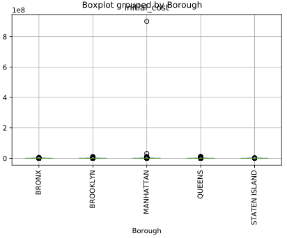
B. Boxplot 箱型圖繪製
可以看見下圖有個明顯的離群值,使整個箱型圖明顯變形。
其中,by 能夠快速使用 .groupby() 的效果,依照 ‘Borough’ 的欄位資料群組化後,觀看 ‘inital_cost’ 的 column= 資料;rot 則可旋轉下方的文字標籤。
# Import necessary modules
import pandas as pd
import matplotlib.pyplot as plt# Create the boxplot
df.boxplot(column='initial_cost', by='Borough', rot=90)# Display the plot
plt.show()
The principle of Tidy Data 整理數據的原則
- 每一個變數(variable)形成一欄
- 每一觀察值(observation)形成一列
- 每一種觀測單位形成一個表格
Tidy Data 的整理方式:
How to convert to tidy data
I. Melt DataFrame
在整理資料時,最重要的便是調整資料的形式,至符合我們要分析的格式;但有時資料的型態並不符合預期,這時就可以靠 melt 來達成我們的願望,簡直就像變魔術xD
# Original Data
       Ozone  Solar.R  Wind  Temp  Month  Day
    0   41.0    190.0   7.4    67      5    1
    1   36.0    118.0   8.0    72      5    2
    2   12.0    149.0  12.6    74      5    3
    3   18.0    313.0  11.5    62      5    4
    4    NaN      NaN  14.3    56      5    5# Melt tb: tb_melt
airquality_melt = pd.melt(airquality, id_vars=['Month', 'Day'])# Melted Data
       Month  Day variable  value
    0      5    1    Ozone   41.0
    1      5    2    Ozone   36.0
    2      5    3    Ozone   12.0
    3      5    4    Ozone   18.0
    4      5    5    Ozone    NaN
        .
        .
        .
  607      9   26     Temp   70.0
  608      9   27     Temp   77.0
  609      9   28     Temp   75.0
  610      9   29     Temp   76.0
  611      9   30     Temp   68.0
上方的案例,利用 id_vars 固定住「Month」和「Day」這兩個欄位,並溶解其他欄位。當然,還有更多的參數能夠控制溶解的方式,可以參考下面寫的文章來操作。
下面再舉一個更詳細的使用過程,melt() 的公式說明:
- id_vars: 固定欄位
- var_name: 顯示分拆後的欄位名
- value_name: 顯示分拆後值的欄位名
因此除了 Month 跟 Day 沒有被溶解外,其他的變數都被轉換到 measurement 的欄位。
# Original Data
       Ozone  Solar.R  Wind  Temp  Month  Day
    0   41.0    190.0   7.4    67      5    1
    1   36.0    118.0   8.0    72      5    2
    2   12.0    149.0  12.6    74      5    3
    3   18.0    313.0  11.5    62      5    4
    4    NaN      NaN  14.3    56      5    5#melting Data
airquality_melt = pd.melt(airquality, id_vars=['Month', 'Day'], var_name='measurement', value_name='reading')# Melted Data
       Month  Day measurement  reading
    0      5    1       Ozone     41.0
    1      5    2       Ozone     36.0
    2      5    3       Ozone     12.0
    3      5    4       Ozone     18.0
    4      5    5       Ozone      NaN
        .
        .
        .
  607      9   26        Temp     70.0
  608      9   27        Temp     77.0
  609      9   28        Temp     75.0
  610      9   29        Temp     76.0
  611      9   30        Temp     68.0
II. Pivot Table Analysis
Pivot_table() 的功能與 melt() 相反,透過交叉檢視資料,從中發現原先資料編排上沒有挖掘到的資訊。詳細的方式可以參考下文,會了這個方式,就能夠挖掘出比一般人更多的洞見。
調整與分割欄位
有時欄位的資料型態,並非我們想要格式。這時透過 str 或 split() 就能按格式切開資料,並整理至另一個新的表格。
Splitting a column with .str
可以發現 variable 的欄位,被分成 gender 和 age_group 兩個欄位。
# Create the 'gender' column
tb_melt['gender'] = tb_melt.variable.str[0]# Create the 'age_group' column
tb_melt['age_group'] = tb_melt.variable.str[1:]# Print the head of tb_melt
print(tb_melt.head())      country  year variable  value gender age_group
    0      AD  2000     m014    0.0      m       014
    1      AE  2000     m014    2.0      m       014
    2      AF  2000     m014   52.0      m       014
    3      AG  2000     m014    0.0      m       014
    4      AL  2000     m014    2.0      m       014
Splitting a column with .split() and .get()
然而有時,資料的分隔並不會都是等距,這時就需要利用 split() 來分拆資料。下列範例利用 .str.split(‘_’) 來分拆資料。
- 透過
.str.split(‘_’)來分拆資料,並放進去 str_split 的欄位 - 透過
str.get()來獲取該欄位 list 中的特定資料 - 分別放至我們想要的欄位裡
# Melt ebola: ebola_melt
ebola_melt = pd.melt(ebola, id_vars=['Date', 'Day'], var_name='type_country', value_name='counts')# Create the 'str_split' column
ebola_melt['str_split'] = ebola_melt['type_country'].str.split('_')# Create the 'type' column
ebola_melt['type'] = ebola_melt.str_split.str.get(0)# Create the 'country' column
ebola_melt['country'] = ebola_melt.str_split.str.get(1)# Print the head of ebola_melt
print(ebola_melt.head())OUTPUT:
        Date  type_country  counts        str_split   type country
    0    289  Cases_Guinea  2776.0  [Cases, Guinea]  Cases  Guinea
    1    288  Cases_Guinea  2775.0  [Cases, Guinea]  Cases  Guinea
    2    287  Cases_Guinea  2769.0  [Cases, Guinea]  Cases  Guinea
    3    286  Cases_Guinea     NaN  [Cases, Guinea]  Cases  Guinea
    4    284  Cases_Guinea  2730.0  [Cases, Guinea]  Cases  Guinea
有效搜尋檔案與資料名稱
如果有很多個檔案可以使用,此時就可以利用套件 glob 來抓取特定的檔案。
- 引進
glob和pandas套件 - 定義
glob的搜尋條件,「*」代表任意的字元並以.csv結尾
# Import necessary modules
import glob
import pandas as pd# Write the pattern: pattern
pattern = '*.csv'# Save all file matches: csv_files
csv_files = glob.glob(pattern)# Print the file names
print(csv_files)# Load the second file into a DataFrame: csv2
csv2 = pd.read_csv(csv_files[1])# Print the head of csv2
print(csv2.head())
Regular expression in cleaning data
有時候最悲慘的是,資料格式並沒有特定的規律,無法使用上述的方式處理。這時強大的正規表達式就出場了!
- 引入 Regular expression 套件
re - 利用
compile來搜尋d(digit) 和 {3} 三個數字(記得索引每個字的時候都要有\來進行定義)。 - 利用
match()來找出相對應的資料。
# Import the regular expression module
import re# Compile the pattern: prog
prog = re.compile('\d{3}-\d{3}-\d{4}')# See if the pattern matches
result = prog.match('123-456-7890')
print(bool(result))# See if the pattern matches
result2 = prog.match('1123-456-7890')
print(bool(result2))
如果要找到特定的數字
透過 \d+ 來搜尋一位數(含)以上的數字,可以看到結果正確搜尋出 [‘10’, ‘1’]。
# Import the regular expression module
import re# Find the numeric values: matches
matches = re.findall('\d+', 'the recipe calls for 10 strawberries and 1 banana')# Print the matches
print(matches)OUTPUT:
['10', '1']
正規表達式的練習,可以參考:W3Cshool|30分钟内让你明白正则表达式入門教程
Checking Data Quality
用 function 來加速清理數據
下面的範例,是為了示範如何把 male 和 female 轉換成 0, 1,並為空缺值替換成 NaN。
另外,使用 apply() 可以放入我們的公式,直接對特定欄位進行操作。
# Define recode_gender()
def recode_gender(gender):# Return 0 if gender is 'Female'
    if gender == 'Female':
        return 0

    # Return 1 if gender is 'Male'
    elif gender == 'Male':
        return 1

    # Return np.nan
    else:
        return np.nan# Apply the function to the sex column
tips['recode'] = tips.sex.apply(recode_gender)# Print the first five rows of tips
print(tips.head())
另一個方式,是用lambda 來清理數據:
其中 apply 所應用的方式,就是前面提到過的正規表達式啦!
# Write the lambda function using replace
tips['total_dollar_replace'] = tips.total_dollar.apply(lambda x: x.replace('$', ''))# Write the lambda function using regular expressions
tips['total_dollar_re'] = tips.total_dollar.apply(lambda x: re.findall('\d+\.\d+', x)[0])# Print the head of tips
print(tips.head())
如果數據重複,就可以用 drop_duplicate():
# Create the new DataFrame: tracks
tracks = billboard[['year', 'artist', 'track', 'time']]# Print info of tracks
print(tracks.info())# Drop the duplicates: tracks_no_duplicates
tracks_no_duplicates = tracks.drop_duplicates()
如果想要用 mean / median 等數字填充:
可以使用 fillna() ,後面加上特定的公式帶入。
# Calculate the mean of the Ozone column: oz_mean
oz_mean = airquality.Ozone.mean()# Replace all the missing values in the Ozone column with the mean
airquality['Ozone'] = airquality.Ozone.fillna(oz_mean)# Print the info of airquality
print(airquality.info())
用 assert 來驗證
如果
assert後面的函示為 false,則會顯示 error。
assert 主要是用來避免當特定的數值可能 Error,導致後面的欄位不會執行。只要 assert 該欄位出現 Error,系統就會報錯,並繼續執行下去。
# Assert that there are no missing values
assert pd.notnull(ebola).all().all()# Assert that all values are >= 0
assert (ebola >= 0).all().all()
Use the pd.notnull() function on ebola (or the .notnull()method of ebola) and chain two .all() methods (that is, .all().all()). The first .all() method will return a True or False for each column, while the second .all() method will return a single True or False.
轉換資料型態
有時會遇到資料型態被預設成 object,這時就能使用 astype() 來轉換資料型態。
# Convert the sex column to type 'category'
tips.sex = tips.sex.astype('category')# Convert the smoker column to type 'category'
tips.smoker = tips.smoker.astype('category')# Print the info of tips
print(tips.info())
df.dtype 檢驗資料型態
# Convert the year column to numeric
gapminder.year = pd.to_numeric(gapminder.year)# Test if country is of type object
assert gapminder.country.dtypes == np.object# Test if year is of type int64
assert gapminder.year.dtypes == np.int64# Test if life_expectancy is of type float64
assert gapminder.life_expectancy.dtypes == np.float64
綜合範例:
- 設定 function 來檢驗資料是否正確。
- 利用 columns[0] 來確認資料欄位是否正確。
- 利用 value_counts()[0] 來檢驗資料是否有不正確地重複。
def check_null_or_valid(row_data):
    """Function that takes a row of data,
    drops all missing values,
    and checks if all remaining values are greater than or equal to 0
    """
    no_na = row_data.dropna()
    numeric = pd.to_numeric(no_na)
    ge0 = numeric >= 0
    return ge0# Check whether the first column is 'Life expectancy'
assert g1800s.columns[0] == 'Life expectancy'# Check whether the values in the row are valid
assert g1800s.iloc[:, 1:].apply(check_null_or_valid, axis=1).all().all()# Check that there is only one instance of each country
assert g1800s['Life expectancy'].value_counts()[0] == 1
大部分的人可能會想像,處理數據分析時會花大部分的時間拉圖表,但很多時候資料的來源是混亂且未經整理的。因此在大部分的時候,可能會花高達 60%~80% 的時間在處理數據,以求資料的精確與清晰。
這篇文章主要是透過 DataCamp 的 Cleaning Data in Python 課程,來紀錄在清洗資料時,可能會遇到的問題,以及可以如何解決它。
如果文中有任何不清楚或是筆誤,都歡迎直接留言跟我說,也歡迎一起討論數據分析的過程!
謝謝你/妳,願意把我的文章閱讀完
如果你喜歡筆者在 Medium 的文章,可以拍個手(Claps),最多可以按五個喔!也歡迎你分享給你覺得有需要的朋友們。